|
1
|
- Project 6 Team
- Phil Coady, Joe Cremaldi,
- John Deas, Steve Escaravage
- February 18, 2009
|
|
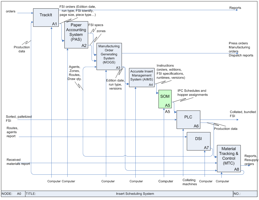
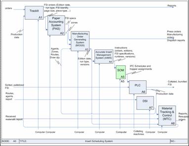
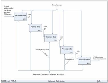
2
|
- Overview of alternative evaluation method
- Introduction to algorithm formulation
- Introduction to business case
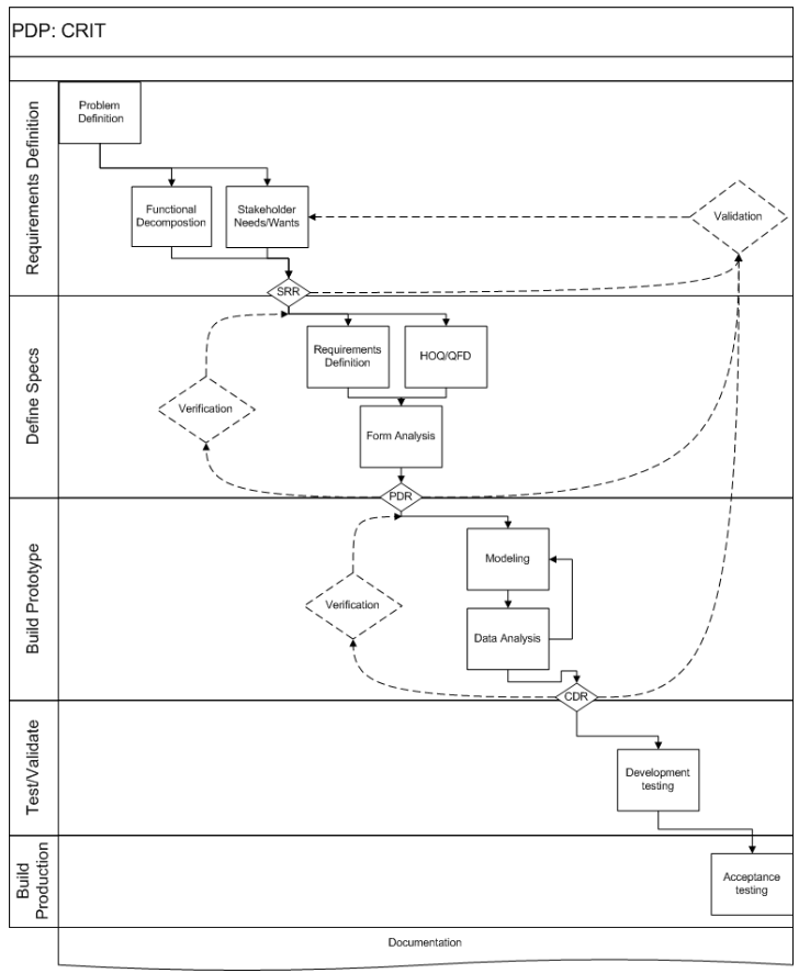
- Appendix 1: Revised functional architecture and PDP
- Appendix 2: Revised schedule and project development plan
|
|
3
|
- Alternative Solution Space is a factorial combination of potential forms
for each function
- Constraints include non-functional requirements of the proposed system,
operational and organizational constraints of the client, and
operational constraints of the delivery team
- In some cases, common sense will be applied to further reduce the
alternative space (i.e., unrealistic options - substantial data entry)
- An Effectiveness Rating, or relative evaluation is required to
differentiate alternatives in terms of performance against functional
requirements
- The Preferred Alternative will be identified through application of an
additive value function of the normalized effectiveness ratings and HOQ
weights
- Throughout the evaluation process, the resulting alternative
instantiations will be evaluated against needs and wants to mitigate
risks
|
|
4
|
|
|
5
|
|
|
6
|
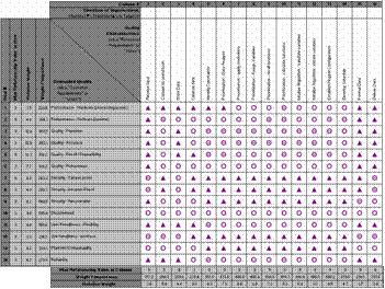
- Note: correlation section of HOQ (roof) not shown
- HOQ weights indicate focus should be directed towards algorithm
development
- Sample relative weight range: 3.8 - 9.3
|
|
7
|
|
|
8
|
- Overview of alternative evaluation method
- Introduction to algorithm formulation
- Introduction to business case
- Appendix 1: Revised functional architecture and PDP
- Appendix 2: Revised schedule and project development plan
|
|
9
|
- Assumptions
- An IPC is defined by an index, a production quantity, an FSI vector
(FSI[]), and an FSI page count vector identifying the number of FSIs at
various page counts FSI_pageCount[]
- Example: IPC X:
[1; 35,000; FSI[0,0,1,0…];
FSI_pageCount [10,6,…]
- The cost function associated with each edge (cij) is a
function of the number and type of hopper change-overs required to
reconfigure the collator from the current IPC to the new IPC
- No cost is associated with open hopper loading time (e.g., if there is
an open hopper available on the collator)
- New hopper assignments will be assigned based on some rule (e.g.,
largest first, smallest first, random)
|
|
10
|
|
|
11
|
- Exact Optimization Methods
- Brute force enumeration infeasible for >20 node networks
- Progressive improvement algorithms support up to 200-225 node networks
- Advanced solutions (cutting plane) currently pushing 10,000+ node tours
but computationally stressing
- Constructive Heuristic Methods
- Generate path through greedy- or insertion- method (e.g., nearest
neighbor/insertion)
- Produces fairly good tour*, with estimates ranging from 1.10x to 2x
optimal tour*
- *For the newspaper problem, we do not need to return to the original
IPC (i.e., solving for path not tour)
- Certain network arrangements result in far from optimal spanning paths
under this method
- Improvement Heuristics
- k-opt approaches start with an initial tour (e.g., developed through
constructive approach) and attempt to improve through removal and
reconstruction of k edges
- Simulated annealing, genetic algorithms, and other artificial
intelligence techniques can be used to drive edge evaluation
- Similar challenges with large networks due to combinatorial enumeration
and evaluation of all sub-tours
- Assessing the Options
- In each case, we can solve the linear optimization relaxation of the
integer problem to get an approximate estimate of “goodness”
- The results can be compared with an assessment of current performance
in the business case to determine acceptance
|
|
12
|
- Overview of alternative evaluation method
- Introduction to algorithm formulation
- Introduction to business case
- Appendix 1: Revised functional architecture and PDP
- Appendix 2: Revised schedule and project development plan
|
|
13
|
- Illustrative Current Operations Example*
- Resource Costs
- 30 shifts labor shifts per week to complete insert production
(10 resources per shift)
- 8 hrs per shift with 75% uptime
(effectively 6 hours per shift)
- Total Production Shift Time = 30*8 = 240 hours
- Production Requirements
- 750,000 insert package demand/wk
- 6,000 packages per hr. line speed
- 750K/6K * (1/.75 uptime) = 167 hrs. required
- Opportunity (Not all can be captured)
- 240 hours - 167 hours = 73 hours ~ 9 shifts
- 9 shifts * 10 resources * $25/hr *8 hrs = $18K
- Assuming 10% capture, then $1800 per week
- Illustrative Technology Augmentation Example*
- Impact of new technology
- Assuming new technology improvements: line speed 10,000 packages per
hour; uptime of 90%
- 750K packages/10K packages per hour *
(1/.9 uptime) = 83 hrs. required
- Opportunity (Not all can be captured)
- 240 hours - 83 hours = 157 hours ~ 19 shifts
- 19 shifts * 10 resources * $25/hr *8 hrs = $38K
- Assuming 10% capture, then $3800 per week
- Business Case Objective
- Develop algorithms to reduce change-over time leading to unnecessary
labor shifts (~$2K opportunity per shift)
|
|
14
|
- Overview of alternative evaluation method
- Introduction to algorithm formulation
- Introduction to business case
- Appendix 1: Revised Functional Architecture and PDP
- Appendix 2: Revised schedule and project development plan
|
|
15
|
|
|
16
|
|
|
17
|
|
|
18
|
|
|
19
|
|
|
20
|
|
|
21
|
|
|
22
|
|

 Notes
Notes