OR 680: Deliverables
George Mason University
Department of Systems Engineering & Operations Research
Spring 2010
Preparing Data for the Model
The data came in large CSV flat files that contain all the data fields as well as, data that was not useful for our model. Before beginning the modeling process we first arranged the data into a more intuitive structure. An options object was created first which parses the data in each row and stores the following information:
- Trading date
- Option type, call or put
- Strike Price (strike price is described as difference from asset price at trading date. To calculate this difference the asset price is first rounded to the nearest integer, then the next greater multiple of 5 becomes the +5 call and the next lesser multiple of 5 becomes the -5 put)
- Expiration date (the raw data file contains only expiration month and expiration year. Since we know that expiration dates fall on the 3rd Friday of each month we can calculate the expiration date)
- Premium
- Days before expiration (this value was calculated by finding the difference between the trading date and expiration date)
- Then the options objects are arranged in a hash map with expiration date as key and options objects as values. Since our model loops by expiration date on the highest level the hash map simplifies searching for the correct data.
Modeling Strategies
Trade and Forget - Trade and forget is the most basic version of strangle that we model. The options writer sells an option and waits until expiration. This is the basis for more advanced strangle strategies. The trade and forget simulates selling strangle for each month and calculating the payoff. The algorithm for all three models can be found in the appendix.
Strangle with Stop-Loss - Strangle with stop-loss adds one layer of complexity to the model. We execute the stop-loss as soon as the market premium price increases by at least the stop-loss value, at which point we buy back the option. To implement stop-loss into the model we need to check the premium price for all trading days between the options writing date and expiration date.
Volatility Driven Decision Making - Volatility driven decision making prevents investors from investing when the market is too volatile. Payoffs can become unpredictable in a volatile market so risk averse investors might not trade until the volatility drops to acceptable levels.
Modeling the Optimal Fractional Investment Allocation
The model sets fractional allocation values, in multiples of 5% from 5% to 100%, and calculates payoffs for the entire period of input data. By limiting fractional allocation values, precision is lost but model run time is gained. Missing values can be estimated since the curve of the function is smooth.
After initializing the trading account as a fraction of capital, the next target is to identify how many options to write or sell. Here the consideration is the largest loss and the margin requirement, which is $5000 for selling an option from the commission. The function can be expressed as follows:
The Number of Contract = The trading account / max(the largest loss, margin)
We compute final payoffs for all fractions for each strategy and identify the fraction with the highest payoff as optimal.
Graphical User Interface
A major component of this project consists of a decision support system for a hypothetical option writer in the form of a graphical user interface (GUI). This interface allows a decision maker to browse returns for all strategies over a selected trading period, along with associated data such as average percent return, optimal fraction of investment, and worst draw-down. The decision maker can filter strategies based on days before expiration, put and call prices, stop-loss value, and maximum volatility. It allows the decision maker to manage risk by filtering strategies that exceed a maximum worst draw-down during the examined trading period, exceed a maximum risk of ruin, or cause the seller's account to dip below a given value.
When the model runs a set of strategies over a given time period, it computes individual trade returns for each strategy along with associated metrics. The output of each trade is written to memory as a data record containing just these values. These data are then saved to a file as a serialized Java object for use later. It is possible to generate and store multiple files with strategies of different types taking place over differing periods of time.
Just as the model and data parsing components, the GUI itself is written in the Java programming language, enabling it to load files written out by the model. Upon start, it loads a user-specified output file from the model containing the trade return data into memory. It then loads the available strategy parameters for days before expiration, put price, call price, stop-loss value, and maximum volatility from the data file into drop-down filters for the user to find strategies. When clicking the filter button, matching strategy data are loaded into a table in the GUI, and allows the user to sort by the available metrics. The user can also select data and copy it into a document or spreadsheet.
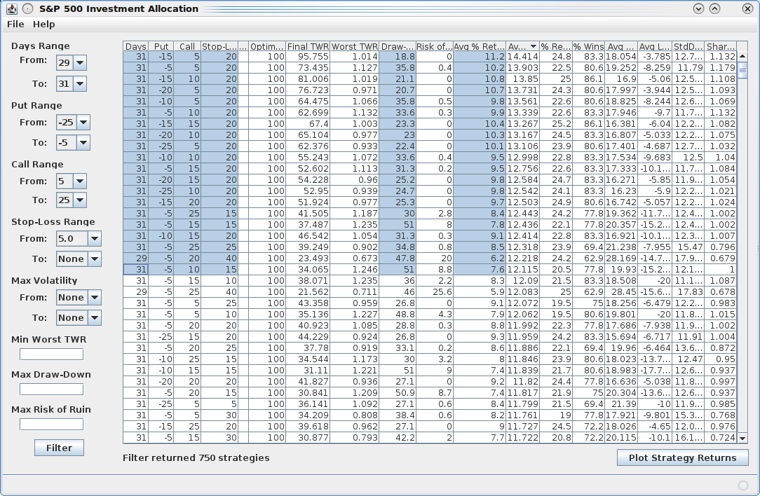
From this window the user can select multiple strategies and compare them by the available statistics. In order to view returns of one or more selected strategies, the user can click on the "Plot Strategy Returns" button. That opens the strangle returns view:
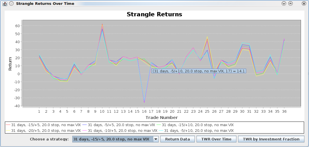
The strangle returns window shows actual simulated returns by trade for each selected strategy. The horizontal axis shows trading opportunities as they occur over time and the vertical axis represents the return from selling this particular strategy. From this window one can select one of the plotted strategies at the bottom and view it's actual return data, terminal wealth relative (TWR) over the trading period, or view the final TWR after trading based on fraction of investment using the respective buttons.
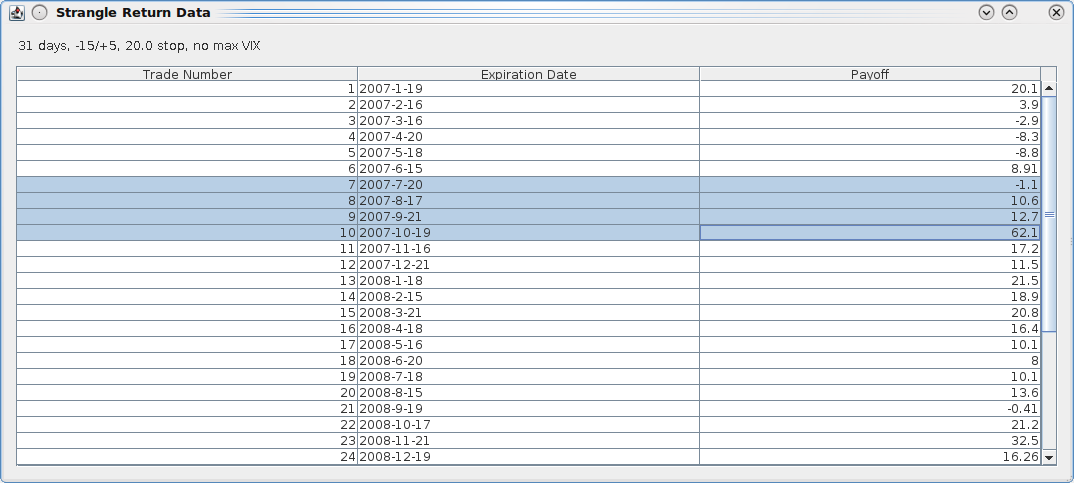
This window shows the actual return data that is displayed for a strategy in the strangle returns window. Each trade has an expiration date associated with it and a payoff on gets for selling it. The payoff accounts for both put and call premiums as well as any stop-loss that is triggered. If a trade cannot be performed, for instance if the trading day is a holiday and has no data, that trade is left out. The payoff values are in points.
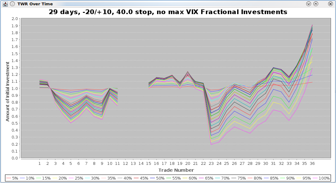
This window shows the TWR of a particular strategy over time. The strategy always starts with a TWR of one, representing the initial investment. The horizontal axis represents trades and the vertical axis is TWR. Each line represents a different fraction of investment. For instance, the first line indexed on the bottom left in the legend refers to the plot of a 5% investment. In the case of this strategy, investing a higher percentage of one's capital gives a lower final return due to the large loss from trade 23.
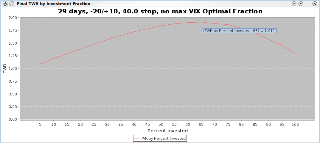
This graph shows the final TWR of based on investment fraction of a given strategy. These are the same data as the final trade of the previous window, and therefore represent the amount of one's initial capital after the entire trading period.
Project Documents
Project Proposal
Progress Report 1
Progress Report 2
Project Presentation
Final Report